Help for data analysis in WebArrayDB |
Currently WebArrayDB is dedicated to the differential analysis. Samples (arrays or specific channels) need to be assigned to different groups for the comparisons among groups. Genes differentially expressed among groups will be generated by the end of analysis.
Tips:
One great feature of WebArrayDB is its capability of cross-platform probe alignment. Probes from different platforms can be aligned by any IDs which were pre-defined as reference ID, such as gene symbol, GenBank ID, RefSeq IDs. After alignment, a data matrix will be made in which each column is from a channel of an array and columns in each row have a same aligned probe/gene. Currently only probes presented in all platforms will be kept in the data matrix for further analysis.
There are six ways to match probes in WebArrayDB:
1) quick alignment,
2) match by “idx” or “unique_id”,
3) match by shared “Reference IDs”,
4) match by “user-specified columns”,
5) match by probe-mapping files,
6) “automatic” match.
In the case that all involved platforms have the same number of probes, all probes are from the printing material sharing the same sequence, and printed in the same order, users can choose quick alignment option. WebArrayDB will actually skip the step of matching and use these platforms as a same one. This might help to save much time since regular alignment can be very time consuming.
The “idx” column contains the printing order (or logical positions) of probes, so probes will be matched by printing order if “idx” is chosen. “unique_id” is the “id” or “unique_id” columns in the probe file.
In order to use “reference IDs” for alignment, users must provide reference IDs in probe files when defined platforms. The steps are:
Probes are considered “identical” if they share the same reference IDs in WebArrayDB. When doing an analysis, users can choose to use one of these reference columns to align probes from different platforms, e.g., RefSeq IDs. That means probes in different platforms with the same RefSeq ID are considered as the same probe. In the eventual data matrix, these probes will be matched in one or more rows, depending on the method to match replicates.
“Identical” probes detected by reference IDs will be assigned a same “cross-platform ID” that is an integer unique in the database. Cross-platform IDs conform to the transitivity and evolution principles and will be used for “automatic” match.
Transitivity: Cross-platform IDs are transitive, e.g., considering probes “A”, “B”, “C”, if A and B share a common reference ID “ref1”, A and B are identical, if meanwhile B and C share reference ID “ref2”, B and C are identical too, then A, B, C are all “identical” and will share a same cross-platform ID.
The method is similar to that by shared “Reference IDs”. But the columns used for matching are not necessarily a reference column names. Theoretically any columns in the probe files can be used for matching. Especially users can select a different column for each involved platform to match probes as if these columns contain referenced IDs from one certain database. This method presents a very flexible way for matching.
Steps to use probe-mapping files:
“Identical” probes detected by probe-mapping files will be assigned a same “mapping IDs” that is an integer unique in the database. Mapping IDs also conform to the transitivity and evolution principles as cross-platform IDs. They will be used for “automatic” match as well.
Users can also choose the “automatic” option, in which WebArrayDB will use existing alignments by probe-mapping files or align probes by all available reference columns including gene_symbol, unique_id and other reference IDs, but the “idx” column in probe file won’t be used.
WebArrayDB will try mapping IDs first, if no matching probes found, try cross-platform IDs again. If still no match, the column “idx” will be used.
When a probe has replicates in one or more involved platforms, he probe alignment among different platforms can be complex due to its many-to-many relationship, including the cases that there are duplicate spots on the array. WebArrayDB has provided six options, "median", "mean", "log mean", "shortest", "longest" and "cartesian product", to deal with multiplex alignments. For example, if two platforms were aligned by RefSeq ID, and one gene is represented by two probes (A1 and A2) in platform A and represented by three probes (B1, B2 and B3) in platform B. When options "median", "mean" and "log mean" were chosen, the median, mean or log mean value of the probes for the same UniGene will be used to represent that gene. If the option "shortest" is chosen, there will be two matches: A1 vs B1, and A2 vs B2. The option "longest" will make one more match in addition to those done for "shortest": A3 vs B3, where "A3" is the log mean value of A1 and A2. For the option "cartesian product", each probes for the same UniGene in Platform A will make a match to all the probes for the same RefSeq in Platform B, resulting in 6 (2 x 3) matches in total for this example.
Normalization is a to minimize systemic noise before implementing differential analysis and is strongly suggested. Users are encouraged to read details about each normalization options before deciding which one to use. In general, there are four steps of normalization.
The first three steps will be done before probe alignment. and the last step will be done after cross-platform probe alignment.
Background correction, within-array normalization and between-array normalization (within platform) are also parts of functions provided in WebArray.
Cross-platform normalization means data normailzation for arrays from different platforms. All between-array normalization methods are included for cross-platform normalization, furthermore, another three cross-platform methods were implemented in WebArrayDB as well:
For the QD normalization, a parameter - “number of bin” has to be set. It is 2, 4, 8, … a number of power of 2. Its default is 8.
For homologous platforms (e.g. different developmental versions of an user-spotted slides with a few probes changed), all between-arrays normalization methods might be used. In such cases, between-array normalization within a platform is unnecessary.
Users have many options in algorithms for differential analysis in WebArrayDB: Student’s t-test, eBayes-moderated t-test, SAM, ANOVA/ANCOVA and non-parametric tests.
Student’s t-test. One of most-widely used statistical method for differential analysis - I assume everybody knows it.
t-test is moderated by empirical Bayes methods and implemented in LIMMA [7, 8]. For two-color array data, users have the options of analyzing the data based on either ratio or intensity. However, if the data or an experiment design are not suitable for a ratio-based analysis, for example, single color array data were included in the analysis, the statistical analysis will be done based on intensity.
SAM represents “Significance Analysis of Microarrays”. This algorithm was developed by Tusher [10].
Mixed-effect model ANOVA plays a very important role in microarray data analysis [1]. This method can deal with multiple factors. The model for ANOVA usually looks like
| E = µ + G + P + A + D + S + ε (1) |
in which E is the observed log-transformed intensity value, µ is the theoretic “real” log-transformed intensity value, G is the group factor, which leads to effects of interests, e.g. treatment effects, P, A, D and S represents effects of platform, array, dye and sample respectively, ε represents the Gaussian random error with 0 as expected value. Under different conditions, there can be more or less factors used in the model. On WebArrayDB, based on data offered by users, platform, array, dye and sample might be considered as factors in which array is considered as a random effect factor.
When using a non-parametric test, Friedman rank sum test, Kruskal-Wallis rank sum test or Wilcoxon rank sum test will be chosen automatically based on the data offered. Specifically, WebArrayDB performs a generalized Friedman rank sum test with replicated blocked data or, as special cases, a Kruskal-Wallis rank sum test on data following a one-way layout or a Wilcoxon rank sum test following a one-way layout with only two groups.
In case that data cannot be treated as blocked/paired, WebArrayDB will omit this option and do a regular analysis based on intensity.
Blocked/paired data has different meaning according to the selected algorithms.
For two-color data, the default behavior of LIMMA is try to use ratio of two channels within array to do statistical analysis. This means data are paired by array. In any other cases, LIMMA will use intensity data for analysis even if you choose to use paired data.
For t-test, SAM test and ANOVA, data might be paired only when there are just two groups defined. In such cases, WebArrayDB try to produce a ratio between the two groups according to selected factor. If this succeeds, ratios will be used for analysis. Then t-test becomes paired t-test. ANOVA will produce a different model based on ratio as well.
When there are just 2 groups, the Wilcoxon rank sum test will be used. If the data between the two groups have intrinsic connections, e.g. from the same array, using same dye, from same sample individual, …we may treated them as paired data, then the test will be done in a paired way.
When there are more than 2 groups, and data among these groups have intrinsic connections, we can treat these data as blocked and Friedman rank sum test will be used, otherwise, it is a Kruskal-Wallis rank sum test.
ANOVA/ANCOVA can be used to investigate the effects of multiple factors/variables. Here variables diff from factors by the type of their values - the values of a variable are number (integer or float) while the type of factors is string even if they consist of digits. Using factors/variables defined by the user or found in the database, a user can define or help WebArrayDB to define the linear model for ANOVA/ANCOVA.
Note that the model will be a mixed-effect model in cast that any random-effect factor/variable are used. Mixed-effect model could be very time-costing in computation.
Factors/Variables falls into three categories:
Based on experiment designs, there are four options to build a model for ANOVA/ANCOVA in WebArrayDB.
In this case, “group” is considered as the only factor that take effects on intensity data. This option is good for simple experiment designs.
WebArrayDB will attempt to use the “group” factor and as many as possible other factors in databases to build a model for ANOVA. Currently the following factors will be tried:
When users select some of these factors, WebArrayDB will try to use them to build a model for ANOVA, any factor that are not suitable will be removed automatically.
WebArrayDB will use the “group” factor and all user-defined factors/variables to build the ANOVA model. This option presents a flexible way for analysis in case that the information in databases in insufficient for specific experiment designs.
There are several significant features/advantages in user-defined model:
This is to describe the comparisons users want to between “groups” . For example, if users put “group2 - group1”, it means the user wants to compare group2 and group1. In the analysis results, M will represent the log base 2 ratio of group2/group1. Multiple comparisons can be separated by “,” or “;”. In default if no information was filled in the Contrast box, all other groups will be compared to the first one, i.e. “group2 - group1; group3 - group1; group4 - group1” if there are total four groups.
Generally, a comparison is defined by group names separated by “+” and/or “-”. Don’t include replicates of a group name within one comparison. But these limitations are removed if you use LIMMA based analysis, which allows more flexible comparisons made by pairs of parenthesis “()”, “/” and numbers, e.g., experienced users can try something like “(group4 - group3) - (group2 - group3)”, or “group3 - (group2 + group1)/2”.
Some other analysis methods that has already been introduced into WebArrayDB, e.g., hierarchical clustering, heatmap, correspondence analysis, between group analysis, and genome or comparative genomic hybridization (CGH) plotting. These analyses can share a common option:
Based on the result of differential analysis, a filter can be defined to screen probes of interests. All probes will be used if no (successful) differential analysis is done. Otherwise users can choose probes by p-values for these analysis. This filter can be optionally used, but it might be necessary for some analyses that cannot handle too many probes, e.g., clustering.
This analysis produces a clustering chart. Depending on the users’ requirements, WebArrayDB can cluster groups or data channels. A successful clustering requires at least three groups or data channels.
This analysis produces a heat map with a two-dimensional clustering. The groups (or data channels) are clustered in the horizontal direction. This should be a cluster chart similar to the “Cluster” above. Probes are clustered on the vertical direction.
COA finds outliers of probes. It requires at least two groups. Please refer to [5, 6].
BGA finds outliers of probes. It requires at least three groups. Please refer to [2, 3].
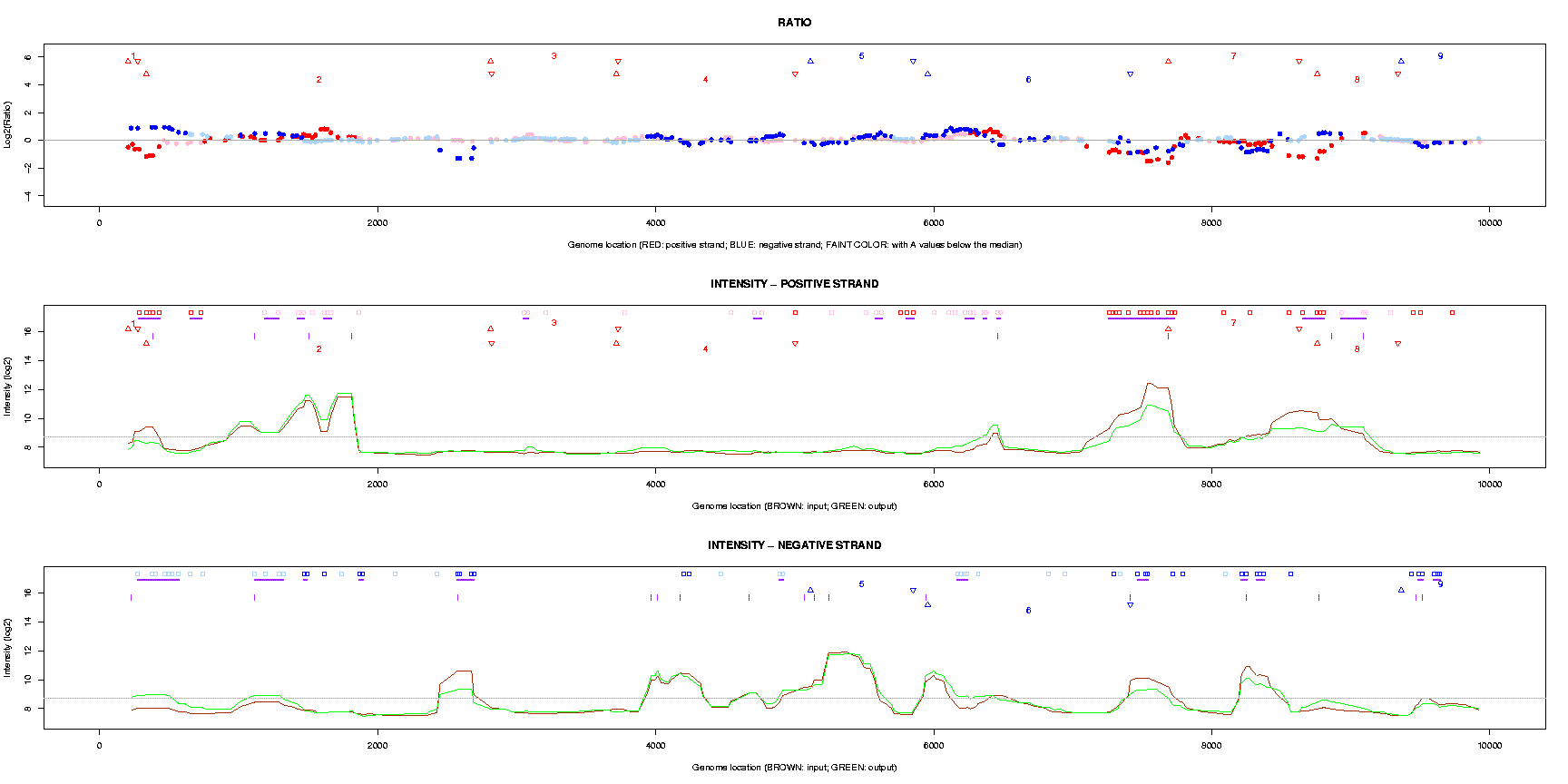
This function is designed for plotting intensity values or ratios along with locations of probes on the genome. Generally, the plotting is based on two-channel data - the first two groups, in which “group1” is used as the green channel (G, or the input channel), and “group2” as the red channel (R, or the output channel).
The main options are listed below.
Plot genome segment
This is good if the probes come from a huge genome. Typically, such a genome is an eukaryotic genome with many chromosomes, e.g. the human genome.
This is good if the probes come from a small genome, e.g., a prokaryotic bacterium genome.
This option does not have much biological significance, but allows data displayed evenly.
At each plotting unit, i.e., a genome segment (see “Plot genome segment” in section 6.5), three charts will be plotted (see Figure 1 and Table 1):
Table 1: Legends for genome plotting
Legend Annotation • Spots indicate the log base 2 transformed ratios for each probe.
Colors are used to indicate probe orientations and significance of p values.red • positive strand, with significant p values pink • positive strand, without significant p values blue • negative strand, with significant p values light blue • negative strand, without significant p values ▵, ▿ Triangles indicate locations of genes. Upwards for start, downwards for end.
The name (or number) between a pair of triangles specifies a gene using “gene_symbol” or a part of it.red ▵, ▿ positive strand blue ▵, ▿ negative strand. ▫ Squares specify locations with significant p values from differential analysis.
Colors are used to indicate probe orientations and regulated direction: output (group2) - input (group1).red ▫ positive strand, down regulated pink ▫ positive strand, up regulated blue ▫ negative strand, down regulated light blue ▫ negative strand, up regulated — Purple horizontal bars indicate adjacent probes associated with significant p values. | Purple vertical bars indicate locations of potential transposons. Curve Intensity values (after log base 2 transformation) of probes along the genome.
Colors are used to indicate probe orientations and regulated direction: output (group2) - input (group1).brown curve the input data (group1) green curve the output data (group2)
The purpose of “transposon analysis” is to identify the location of transposons on the genome. This analysis can be carried out only when the nucleic acids for hybridization were amplified by primers on transposons. Meanwhile the probe file for involved microarray platform must contain necessarry information for genome ploting.
Transposon analysis is done on the basis of genome plotting (see section 6.5). While all options in section 6.5 are applicable for transposon analysis, two additional options are used as well:
Transposon analysis outputs “genome plotting” (see Figure 1) with vertical bars indicating locations of transposons (see Table 1).
Five additional TAB-delimited files will be created too:
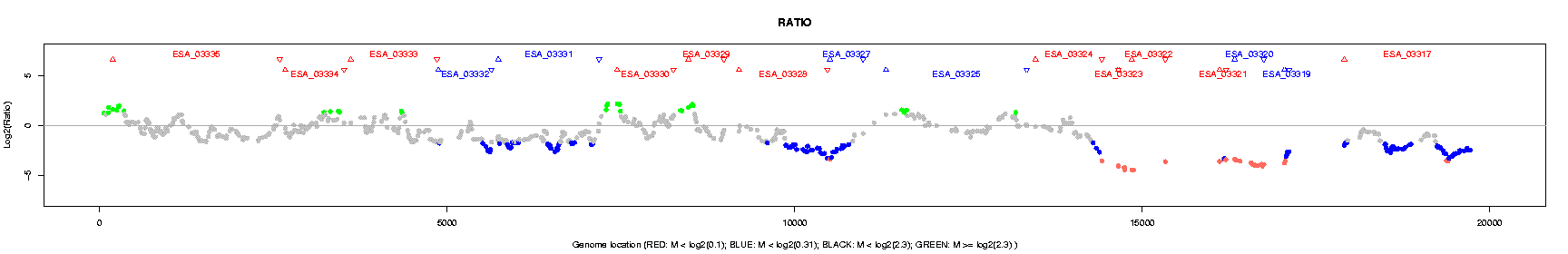
The users can set up three break points to make four intervals (spaces) for the ratios. Ratios in different spaces will be plotted in distinguished colors: RED, BLUE, GRAY, and GREEN.
Bacterium CGH analysis outputs a little different “genome plotting”, only ratios are plotted (see Figure 2). The differences in legends are also listed in Table 2.
Table 2: Legends for bacterium CGH plotting
Legend Annotation • Spots indicate the log base 2 transformed ratios for each probe.
Colors are used to indicate probe orientations and significance of p values.red • ratios below the first (lowest) break point. blue • ratios between the first two break points. gray • ratios between the last two break points. green • ratios above the last (highest) break point.
An additional TAB-delimited file with the name ended with “bacCGH_table.txt”, is produced with gene-wise (by “gene_symbol”) summary for number of probes, and intensity values (log base 2 transformed).
Some global options can be defined in this section.
EPS chart format
Here is an example for using technical replicates. Assume a project involved three biological replicates of two conditions (i.e. 6 samples in total) which were compared on arrays, two channels, condition 1 versus condition 2. They also dye-swapped every sample, so now we end up with six arrays with two channels each, each sample has two technical replicates:
| samples for condition 1: A1, A1, A2, A2, A3, A3 |
| samples for condition 2: B1, B1, B2, B2, B3, B3 |
We will explain how to use ANOVA and eBayes-moderated t-test (in LIMMA) to compare the difference of samples between the two conditions.
Create two groups with samples in order:
| group1: | A1, A1, A2, A2, A3, A3 |
| group2: | B1, B1, B2, B2, B3, B3 |
Choose the third option for ANOVA model - Use following user-defined factors as well as "Group", and define a factor with the following values:
| Factor name: facsamp |
| Factor type: random |
| Data type: string |
| Factor values: A1, A1, A2, A2, A3, A3, B1, B1, B2, B2, B3, B3 |
Create six groups:
| group1: | A1, A1 |
| group2: | A2, A2 |
| group3: | A3, A3 |
| group4: | B1, B1 |
| group5: | B2, B2 |
| group6: | B3, B3 |
Comparisons to make is:
(group4 + group5 + group6 - group1 - group2 - group3)/3
This document was translated from LATEX by HEVEA.