Summary
We compared the performance of 41 analysis models based on 14 software packages and different datasets, including high-quality data and low-quality data from 33 species. In addition, computational efficiency, robustness, and joint prediction of the models were explored. As a practical guidance, key points for lncRNA identification under different situations were summarized. In this investigation, no one of these models could be superior to others under all test conditions. The performance of a model relied to a great extent on the source of transcripts and the quality of assemblies. As general references, both FEELnc_all_cl and CPAT_mouse work well in most species, and CNCI_ve performs better with incomplete transcripts in non-model organisms, while COME, CNCI, and lncScore are good choices for model organisms. Since these tools are sensitive to different factors such as the species involved and the quality of assembly, researchers must carefully select the appropriate tool based on the actual data.
Results
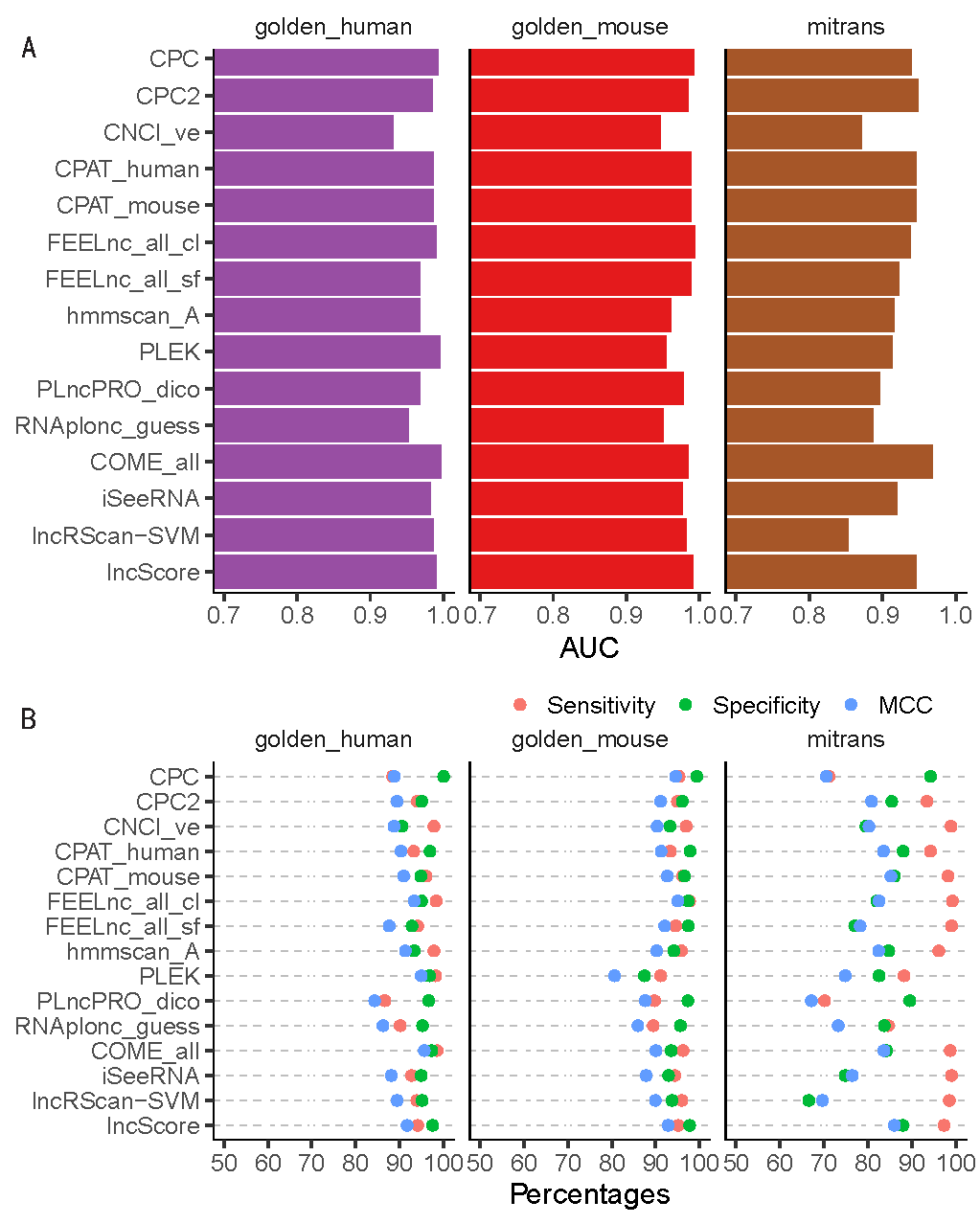
The representative models are a subset of the models been tested. (A) AUC value of ROC curve for each model on golden_human (red), golden_mouse (green), and mitrans (blue). (B) Sensitivity (red), Specificity (green), and Matthews correlation coefficient (MCC, blue) values for each model on the testing data. Sensitivity indicates the proportion of true classified positive samples (lncRNAs) on the total input positive samples (in percentage). Specificity indicates the proportion of true classified negative samples (mRNAs) on the total input negative samples (in percentage). MCC indicates the overall performance ranges from -100 to 100 (in percentage), where 100 implies a perfect prediction, 0 implies a random prediction, and -100 implies a totally wrong prediction.
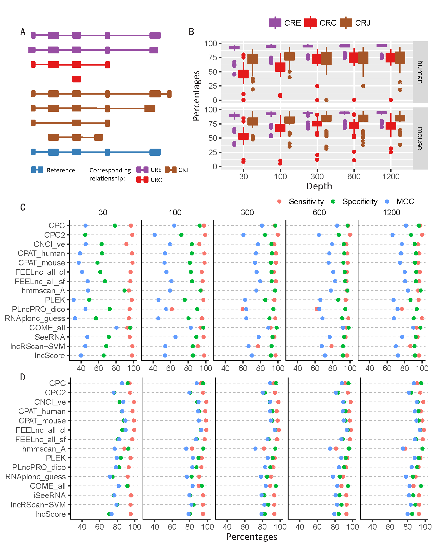
Based on the golden-standard sequence sets (golden_human and golden_mouse), simulated Illumina sequencing data sets were generated by Polyester with five sequencing depths: 30X (which means that averagely 30 reads were simulated from each transcript), 100X, 300X, 600X, and 1200X. (A) The relationship between assembled transcripts and its templates. CRE transcript shares an identical intron chain with its template; CRC transcript is covered by its template; CRJ transcript shares at least one splicing site with its template. (B) Box plots for the MCC of all testing models on the simulated data of different sequencing depths. (C) Performance of representative models on human CRC transcripts. (D) Performance of representative models on human CRJ transcripts.
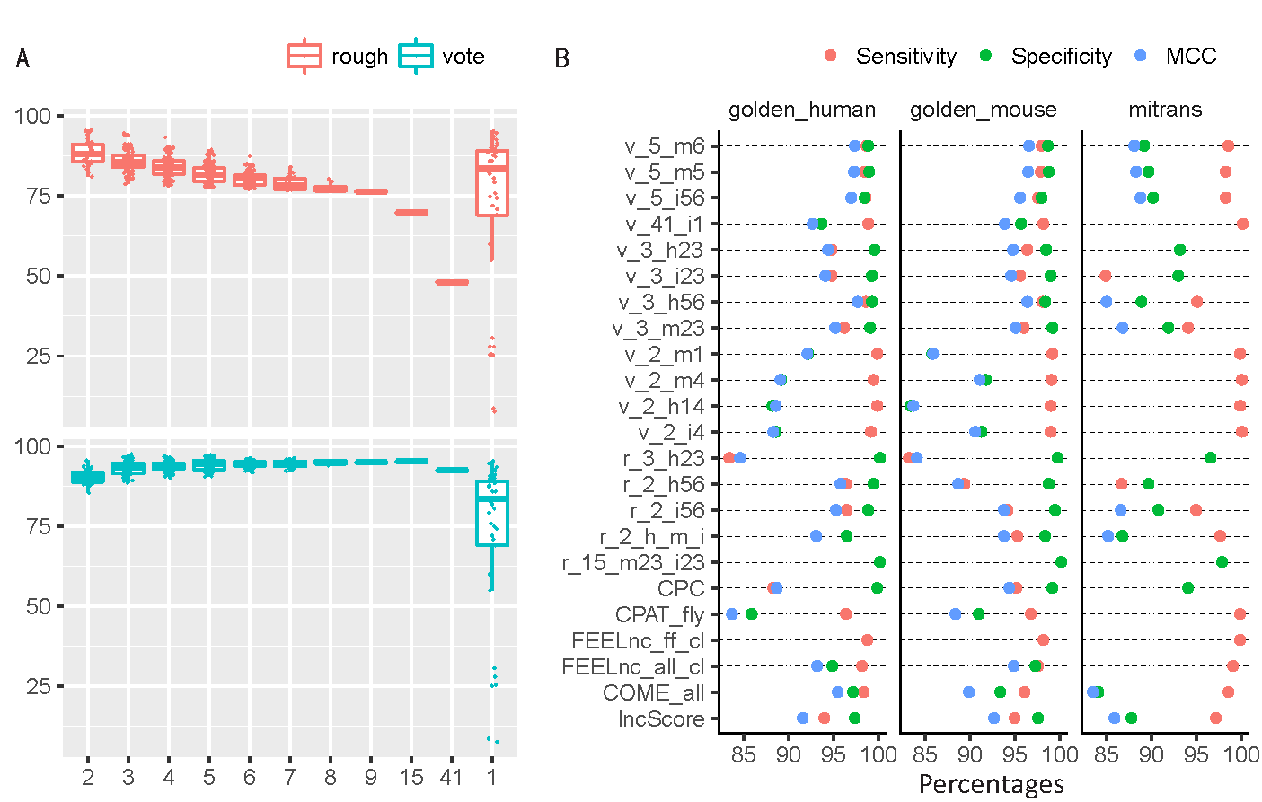
(A) The MCC of joint predictions with different number of models on the golden_human data. The combination methods ("rough" and "voting") were described in the "Methods" section. (B) Comparison of optimal joint predictions and optimal single models on three datasets (golden_human, golden_mouse, and mitrans). The optimal model is defined as one joint/single prediction performed best in terms of any metric of Sensitivity, Specificity, positive predictive value (PPV), negative predictive value (NPV), Accuracy, and MCC on any dataset. The names of joint prediction follow such rule: (combination method, v for vote and r for rough)_(the number of models were used in combination)_(descriptions, where characters represent datasets: h for golden_human, m for golden_mouse, and i for mitrans; numbers 1-6 represent Sensitivity, Specificity, PPV, NPV, Accuracy, and MCC respectively). For example, r_15_m23_i23 means 15 models were conbined in the joint prediction following the rough rule, and this prediction showed best Specificity and PPV on golden_mouse data as well as on mitrans data. Particularly, r_2_h_m_i is the abbreviation of r_2_ h14_m1456_i14 which were two-model joint prediction that have best Sensitivity and NPV on golden_human; Sensitivity, NPV, Accuracy, and MCC on golden_mouse; Sensitivity and NPV on mitrans. The complete list of models used in combination were recorded in Supplemental Table S15.
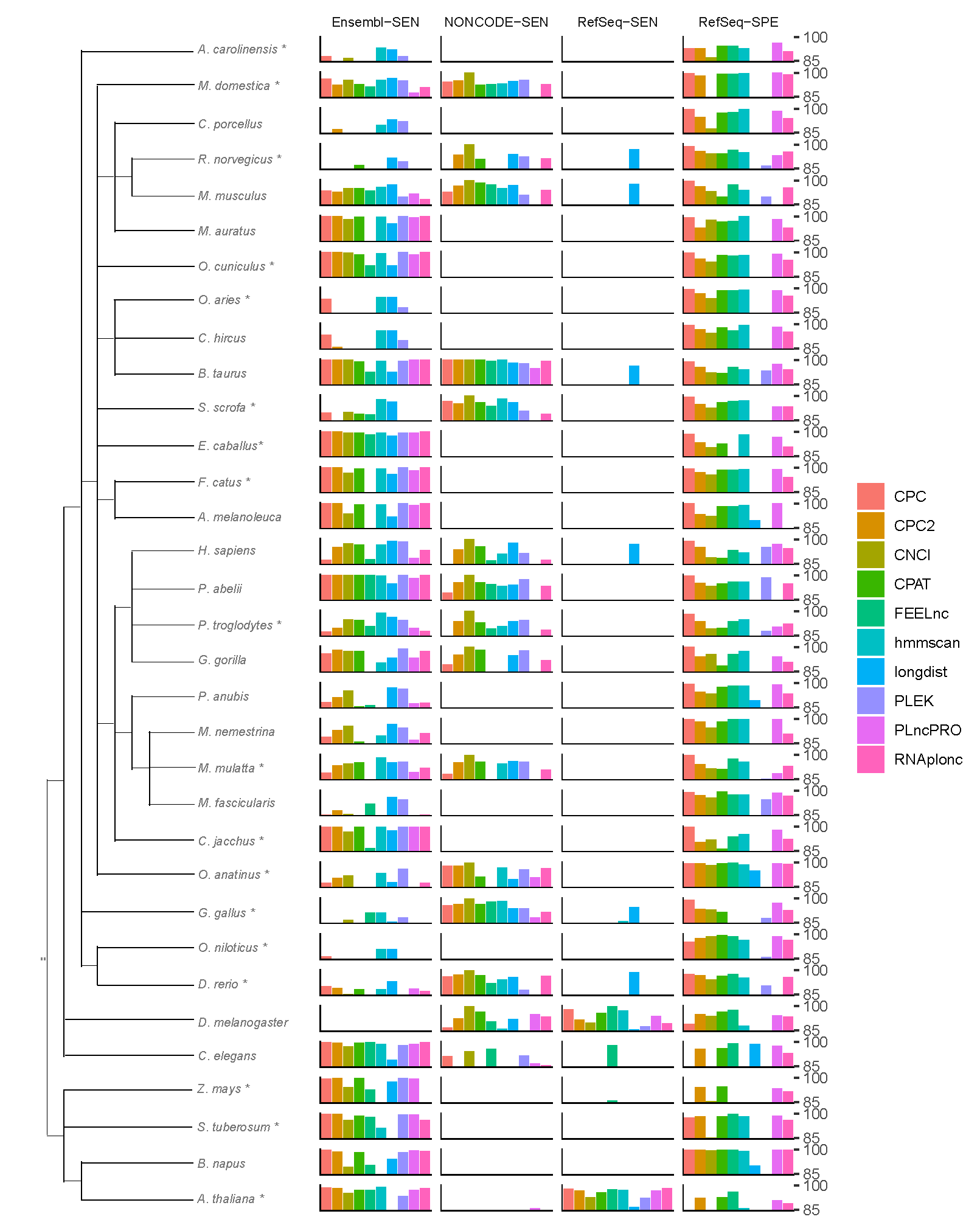
The tree on the left depicts the taxonomy of the species involved, regardless of the evolutionary distance. The sampling procedure for core species (labeled with *) and peripheral species is described in the "Methods" section. For each species, this plot displays the optimal model with regard to the four metrics: Sensitivity on Ensembl, NONCODE, RefSeq, and Specificity on RefSeq. The best prediction for multiple-model-software was showed.
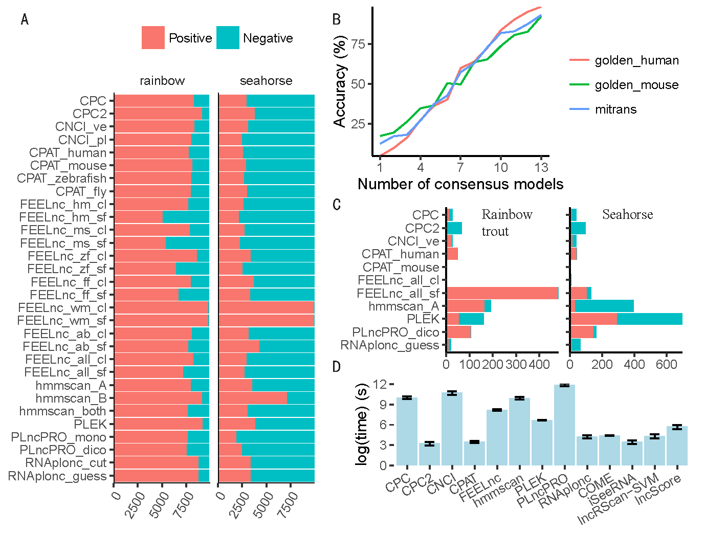
(A) Prediction bias. This figure shows the counts of positive (red) and negative (blue) results predicted by each model in addition to the longdist-based models. (B) The relationship between Accuracy and the count of models that give consensus predictions. Representative models were used in this analysis. (C) The counts of positive and negative disagreed-predictions on rainbow trout (left) and seahorse (right) respectively. The transcripts that were reported positive by one model while negative by others of representative models were regarded as positive disagreed-predictions and vice versa. (D) Average time consumption of each software tool for predicting 5,000 transcripts on golden_human, golden_mouse, and mitrans. The error bar shows the 95% confidence interval of Gaussian distribution.
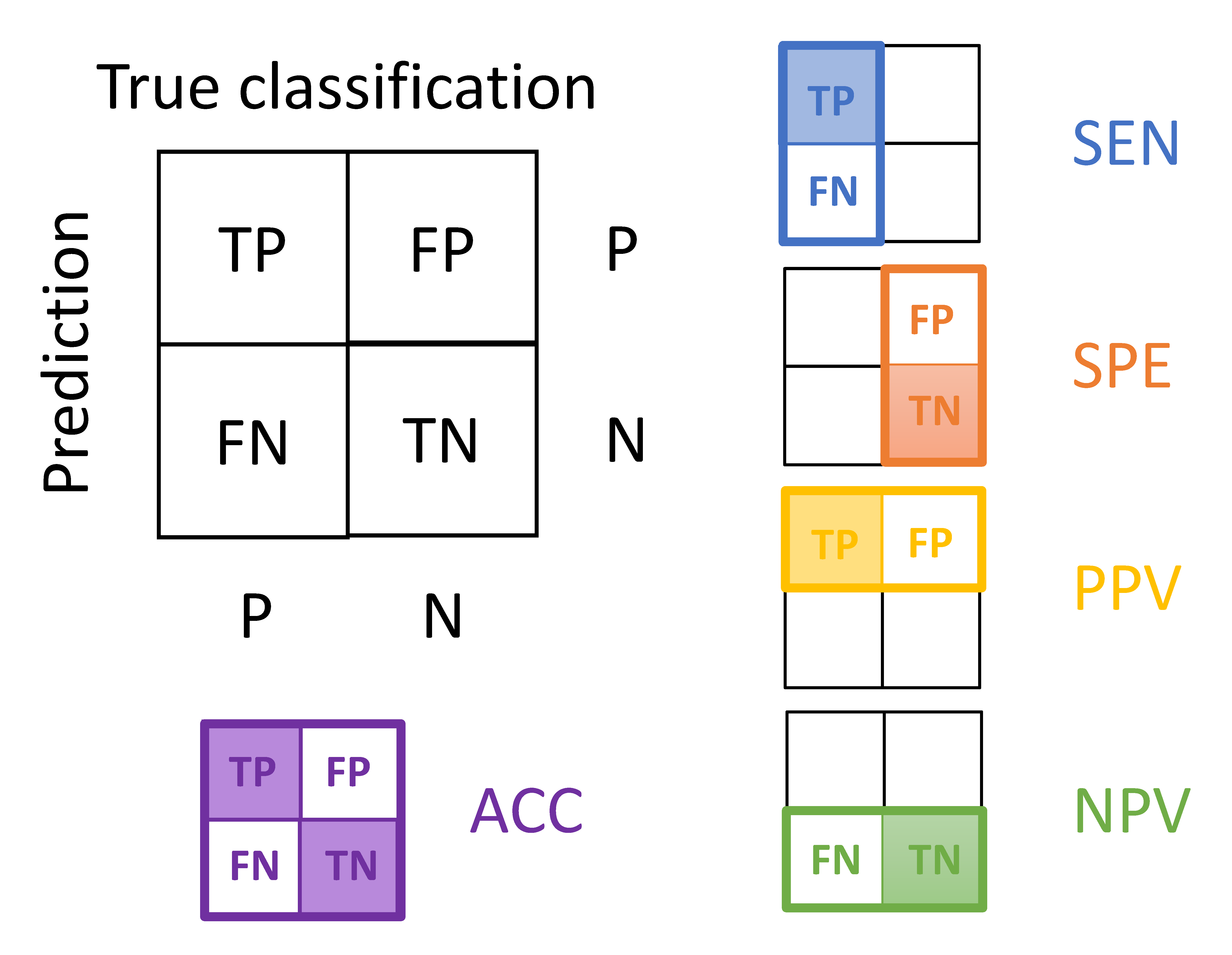
The value is calculated by dividing the predicted count in the shadowy box by the predicted count in the whole rectangle (or square) with a colored border.